Switching from Matlab to Python
Switching from Matlab to Python
by Nick Cortale
This guide will hopefully ease the transition from matlab to python. Most of this post was taken from Jake Vanderplas’s “Introduction to Python” notebooks that he wrote for his ASTR 599 class. You can find the full list of notebooks here.
This guide is also not going to try to convince you to switch from matlab to python. I’m assuming you’ve seen the light and want to make the switch. If you do want to read a little bit, here are a couple of articles:
Python Architecture
Matlab is set up quite nicely. Everything is integrated extremely well and everything plays nicely together. Python, on the other hand is open source and consequently has many different packages written by many different people that can be used at any one time.
To reproduce the matlab environment in python you need two main packages:
- Numpy - matrix library and a lot more
- Matplotlib - a plotting library
Alright. Let’s get into it.
Downloads
The first thing you will need to do is download the anaconda package manager. This installs everything you will need in the scientific stack –or mostly everything. This can be thought of as installing all the matlab toolboxes (except you will not need to pay thousands of dollars). Anaconda has made working with numerous python packages extremely simple. The user no longer has to worry about dependencies and updating or downgrading packages to work with other packages. Anaconda is truly amazing. This download will also include the jupyter notebook, which is where I do a lot of my data analysis and prototype ideas.
There is also some debate about whether to use python 2 or python 3. A year ago I would have recommended python 2, but at this point I would recommend python 3. I have made the switch with no plans to go back. Check out this post for more information.
The next thing you will want to download is a text editor. This is where you will write your functions, classes, and anything else you could want. I like sublime text or atom, but there are others out there that you can experiment with.
Education
There are a ton of resources out there for those switching from Matlab to python. The documentation for python packages is great. There are tons of examples and explanations about everything you could want. If you feel like the documentation isn’t working out for you, simply googling something like “linspace in python” or “xlim in python” will usually get you what you need. Here are some resources to get you started.
Packages
Like I’ve mentioned, there are two core packages –you can think of them like toolboxes –that reproduce most of the core Matlab package. They are matplotlib, which is a plotting environment, and numpy, which is a matrix multiplication library as well as much more. Some other interesting packages are Scikit Learn for machine learning and Pandas for data manipulation and time series analysis.
Alright. Lets get into it!
Comapring code
1
2
3
4
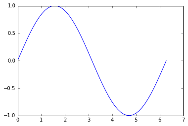
%some matlab code
x = linspace(0,2*pi);
y = sin(x);
plot(x,y)
1
2
3
4
5
6
7
8
9
#Some python code
import matplotlib.pyplot as plt
import numpy as np
%matplotlib inline

x = np.linspace(0,2*np.pi)
y = np.sin(x)

plt.plot(x,y)
Okay, so the first obvious difference is the import at the top of the code. Since python has such a huge open-source ecosystem, we have to tell python which packages we wish to use. The matplotlib.pyplot is our plotting library and the %matplotlib inline is called a magic. Don’t worry about it too much. It allows us to have “inline plots” or plots displayed directly in our jupyter notebook.
Also notice the np. before linspace, pi, and sin. This tells python that we want to use the numpy versions of those functions. For example, there are different implementations of min and max in numpy than in base python. The same thing goes for plt..
Coding python
Here we are just going to get our feet wet in some basic python sytax and see how it differs from matlab. Here is a roadmap:
- Print Hello World / Print Variables
- Integers vs Floats
- Indentation Matters
- Comparisons of Strings/Numbers
- Flow Control: Conditionals and Loops
1. Print Hello World / Print Variables
1
print("Hello World")
> Hello World
1
2
3
4
5
6
7
a = 4
b = 6
c = a/b

print('a =', a)
print('b =', b)
print('c =', c)
> a = 4
> b = 6
> c = 0.6666666666666666
2. Integers vs Floats
Python 3 does division as you would expect coming from matlab. Python 2, however, treats floats and integers differently. For example in python 2 if you did 4/6 it would return 0 . Python 3 changed this. For example in python 3:
1
2
3
4
a = 4
b = 6
c = a/b
print(c)
> 0.66666666
Just something to keep in mind if you ever have to work in python 2.
3. Indentation Matters
Unlike Matlab, python cares about white space. Instead of having end after a for-loop, python uses white space. This means that you have to be careful to adhere to python’s syntax. This counts for both spaces and tabs.
1
2
3
# tab
a = 4
    b = 6
> IndentationError: unexpected indent
4. Comparisons of Strings and Numbers
This is the same in matlab as it is in python.
1
2
3
4
5
6
a = 4
b = 6

print(a == b)
print(a != b)
print(a == b-2)
> False
> True
> True
Be Careful with floating point numbers
Due to differences in absolute accuracy, the two wont be the same. For example it might be 0.30000002032 == 0.30000000392 or something.
1
(.1 + .2) == .3
> False
5. Flow Control: Conditionals and Loops
Again, white space is very important here. Instead of using “ends”, python utilizes indents.
1
2
3
4
5
x = 1
if x > 0:
    print("yo")
else:
    print("dude")
> yo
6. Functions
Functions work similarly in python as they do in matlab. You can put a bunch of them at the top of your script (or bottom, but that is bad python style). Again, watch your whitespace.
1
2
3
4
5
def addnums(x, y):
    return x + y

result = addnums(1, 2)
print(result)
> 3
Keywords are also extremely useful to use in function definitions. I use them in just about every function I write.
1
2
3
4
5
def scale(x, factor=2.0):
    return x * factor

print(scale(4))
print(scale(4,factor=10))
> 8.0
> 40
Functions have own variables
It doesn’t matter what is in your workspace. A function is self-contained. The same as Matlab.
1
2
3
4
5
6
7
8
9
def modify_x(x):
    x += 5
    return x

x = 10
y = modify_x(x)

print(x)
print(y)
> 10
> 15
Modules
You might have a bunch of useful functions that you want to import and use within your script, but don’t want them to be in the same script. No worries! You can simply import them as long as they are in the same working directory. For example you might have the file mymodule.py and within that file you have two functions:
1
2
3
4
5
6
7
def add_numbers(x, y):
    """add x and y"""
    return x + y

def subtract_numbers(x, y):
    """subtract y from x"""
    return x - y
You can import these functions like so:
1
2
3
4
import mymodule as MM

print('1 + 2 =', MM.add_numbers(1, 2) )
print( '5 - 3 =', MM.subtract_numbers(5, 3))
> 1 + 2 = 3
> 5 - 3 = 2
Part 2: Closer to Matlab
Now that we have some of the syntax down, we can move onto numpy and matplotlib. You should feel more at home here as these two packages are extremely similar to matlab syntax except for a few python quirks.
1. Numpy
Numpy is going to be used for the majority of your code. Most of these functions should seem familiar.
1
2
3
4
5
6
import numpy as np

x = np.zeros(5)
x2 = np.ones(x.shape)
print(x)
print(x2)
> array([ 0., 0., 0., 0., 0.])
> array([ 1., 1., 1., 1., 1.])
Multidimensional
1
2
3
#notice the tuple
y = np.zeros((5,5))
print(y)
[[ 0.,  0.,  0.,  0.,  0.],
 [ 0.,  0.,  0.,  0.,  0.],
 [ 0.,  0.,  0.,  0.,  0.],
 [ 0.,  0.,  0.,  0.,  0.],
 [ 0.,  0.,  0.,  0.,  0.]])
1
2
x = np.random.rand(5,5)
print x
[[ 0.44403323  0.53621646  0.18661027  0.55444589  0.13948141]
 [ 0.14632214  0.80706578  0.67579172  0.8154011   0.72703239]
 [ 0.31724671  0.69672609  0.81298429  0.72622235  0.38256724]
 [ 0.34576417  0.54684503  0.59555949  0.07682714  0.18278758]
 [ 0.83063867  0.65786224  0.05077883  0.47636297  0.5422061 ]]
Shapes and Indexing
One of the biggest differences for me was the difference between a shape that is (5,1) and one that has a shape of (5,). These are not the same in numpy and the shape of (5,) does not even exist in matlab.
1
2
3
4
5
x1 = np.random.rand(5)
x2 = np.random.rand(5,1)

print(x1.shape)
print(x2.shape)
> (5,)
> (5,1)
Creating Masks
Masks are created the sameway in python as they are in matlab.
1
2
3
4
x = np.arange(16)
mask = x>10

print(x[mask])
> [11 12 13 14 15]
Indexing
Another huge difference is indexing. The indexing in python starts at zero for the first element. This definitely takes some getting used to, but has its advantages in the long run–or so I think it does.
1
2
3
4
5
x = np.array([10,20,30,40,50,60,70])

print(x[0:2])
print(x[2:4])
print(x[4:])
> [10 20]
> [30 40]
> [50 60 70]
1
2
3
4
5
6
x = np.arange(16).reshape(4,4)

print(x)
print(x[2])
print(x[:,2:4])
print(x[2:])
> [[ 0  1  2  3]
  [ 4  5  6  7]
  [ 8  9 10 11]
  [12 13 14 15]]

> [ 8  9 10 11]

> [[ 2  3]
  [ 6  7]
  [10 11]
  [14 15]]

> [[ 8  9 10 11]
  [12 13 14 15]]
Views are not copies
Matlab creates copies of everything and this makes it sometimes very inefficient. Python creates a view into an array. This means that it is not an actual copy, but just a pointer to the other array. This is a little confusing until you see it in action
1
2
3
4
x = np.arange(8)
x_2 = x.reshape(2, 4)
print(x)
print(x_2)
> [0 1 2 3 4 5 6 7]

> [[0 1 2 3]
  [4 5 6 7]]
1
2
3
x[0] = 1000
print(x)
print (x_2)
> [1000    1    2    3    4    5    6    7]

> [[1000    1    2    3]
   [   4    5    6    7]]
We can see that although we only modified x, x_2 was also changed.
Properties and Methods
Instead of calling a function, you can use dot notation to get information about a matrix or perform some basic operations.
1
2
3
4
5
print ('Data type                :', x.dtype)
print ('Total number of elements :', x.size)
print ('Number of dimensions     :', x.ndim)
print ('Shape (dimensionality)   :', x.shape)
print ('Memory used (in bytes)   :', x.nbytes)
> Data type                : int64
> Total number of elements : 8
> Number of dimensions     : 1
> Shape (dimensionality)   : (8,)
> Memory used (in bytes)   : 64
1
2
3
print('Minimum and maximum :', x.min(), x.max())
print('Sum and product of all elements :', x.sum(), x.prod())
print('Mean and standard deviation :', x.mean(), x.std())
> Minimum and maximum             : 1 1000
> Sum and product of all elements : 1028 5040000
> Mean and standard deviation     : 128.5 329.401350938
Matrix Operations
Most of these are the same as Matlab. The only difference is that multiplying defaults to element by element.
1
2
3
4
5
a = np.random.randint(0,10,size=(4,4))

print(a)
print(a*a) #element by element
print(a@a) #matrix multiplication
> [[3 4 2 1]
  [2 4 2 1]
  [1 2 3 2]
  [3 3 3 4]]

> [[ 9 16  4  1]
  [ 4 16  4  1]
  [ 1  4  9  4]
  [ 9  9  9 16]]

> [[22 35 23 15]
 [19 31 21 14]
 [16 24 21 17]
 [30 42 33 28]]
2. Matplotlib
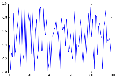
Most of the syntax for plotting is very similar to matlab.
1
2
3
%matplotlib inline  #only include if in jupyter notebook
import matplotlib.pyplot as plt
plt.plot(np.random.rand(100));
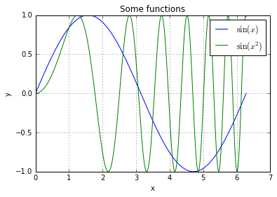
Here’s a longer example with most of the stuff that you could want to do to a plot.
1
2
3
4
5
6
7
8
9
10
x = np.linspace(0, 2*np.pi, 300)
y = np.sin(x)
y2 = np.sin(x**2)
plt.plot(x, y, label=r'$\sin(x)$')
plt.plot(x, y2, label=r'$\sin(x^2)$')
plt.title('Some functions')
plt.xlabel('x')
plt.ylabel('y')
plt.grid()
plt.legend();
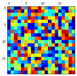
Figuresize and linewidth
1
2
a = np.random.rand(20,20)
plt.matshow(a)
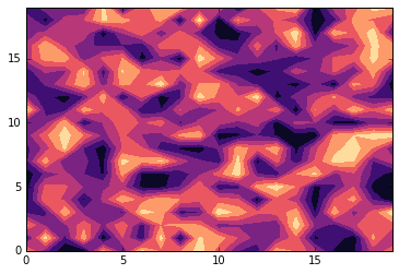
1
plt.contourf(a,cmap='magma')
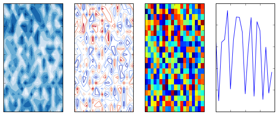
Subplots are a little confusing to understand, but what is happening is that you are creating four axis and the plotting something on each of them.
1
2
3
4
5
6
7
8
fig, axes = plt.subplots(1,4, figsize=(10,4))
axes[0].contourf(a, cmap='Blues')
axes[1].contour(a, cmap='coolwarm')
axes[2].pcolor(a, cmap='jet')
axes[3].plot(a[1]);
for ax in axes:
    ax.set_xticklabels([])
    ax.set_yticklabels([])
Conclusion
Well that is pretty much it. I hope switching to python is a little less daunting.
Feel free to contact me with questions, suggestions, or something you would like me to add!