Exploring TSNE with Bokeh

Introduction

This post explores the TSNE algorithm and its tunable hyperparameters. To keep the blog post clean, the majority of the code was left out of this post, however, you can check out the jupyter notebook that contains all the code for this post.

If you’ve never heard of TSNE before, you might want to check out the following links.

1. Video - 3 min - Explains the difficulty of visualizing high dimensional space.
2. Video - 12 min - Explains the TSNE algorithm at a high level.
3. Article - Interactive visualizations and how to use TSNE effectively.
4. Paper - The original paper describing TSNE.
5. Code - Scikit-Learn’s implementation of TSNE.

If you’re note convinced that TSNE is cool, check out some of these visualizations below.

Digits Data Set

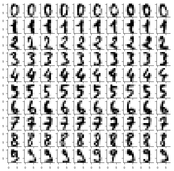
In order to explore this dimensionality reduction technique, we will use the same data as explored in this scikit-learn example. That example, however, compares different manifold learning algorithms and we will instead focus on only tsne. The digit dataset can be loaded in as shown below. Notice that we also normalize each sample, so each plot takes on values between 0 and 1.

1
2
3
4
5
6
7
8
X, y = datasets.load_digits(return_X_y=True)
X = preprocessing.normalize(X)

fig, ax = plt.subplots(10,10, figsize=(10,10), sharex=True, sharey=True)
for i in range(10):
    for j,samp in enumerate(X[y==i][0:10]):
        ax[i,j].imshow(samp.reshape(8,8))
sns.despine()

Next we put this dataset into scikit-learn’s implementation of TSNE. We then visualize the results of TSNE using bokeh. Select the mouse-wheel icon to zoom in and explore the plot.

1
2
tsne = manifold.TSNE(n_components=2, init='pca', random_state=0)
x_tsne = tsne.fit_transform(X)

One of my favorite things about the plot above is the three distinct clusters of ones. There is a cluster of ones that are just a straight vertical line, another cluster with just a top, and a third cluster that has both a top and a bottom line. Another interesting point is the infiltration of a three into the sevens. Looking at that example, it does appear to resemble a seven.

Exploring Hyperparameters

Next we see how hyperparameters effect the resulting dimensionality reduction. Specifically, we look at the following hyperparameters:

1. Initialization
2. Perplexity
3. Learning Rate
4. Iterations
5. Random State
6. Early Exaggeration

1. Initialization

init : string or numpy array, optional (default: “random”)

Initialization of embedding. Possible options are ‘random’, ‘pca’, and a numpy array of shape (n_samples, n_components). PCA initialization cannot be used with precomputed distances and is usually more globally stable than random initialization.

The algorithm can be initialized with either PCA or a random initialization. The documentation from scikit-learn and the resulting plot is shown below.

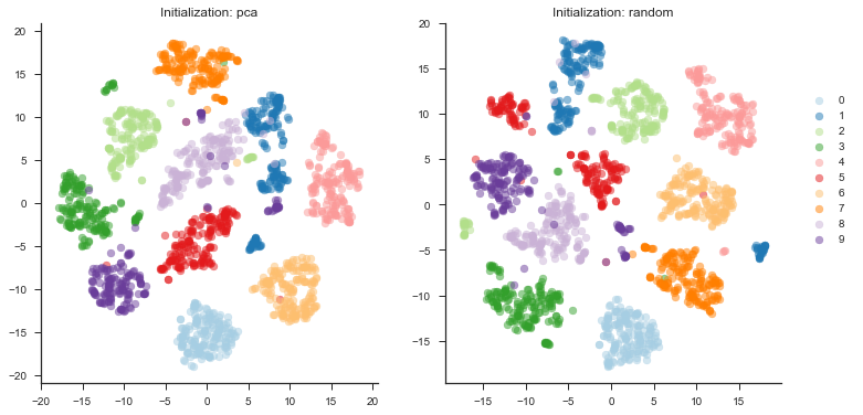
As we can see from the plot above, the initialization in this case does not really have an effect on the outcome. For larger datasets, however, it is recommended to initialize with a PCA.

2. Perplexity

perplexity : float, optional (default: 30)

The perplexity is related to the number of nearest neighbors that is used in other manifold learning algorithms. Larger datasets usually require a larger perplexity. Consider selecting a value between 5 and 50. The choice is not extremely critical since t-SNE is quite insensitive to this parameter.

Perplexity is roughly related to how many near neighbors you expect to see around a point. For example, in a densely populated space, you would want to choose a higher value to more efficiently segment the space.

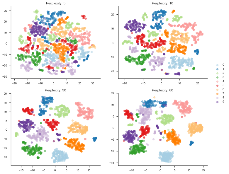
As we can see from the plot above, choosing a reasonable perplexity value is critical. As the perplexity is increased the groupings become tighter and more meaningful for this dataset. Without being quantitative, a perplexity value of 30 appears to most efficiently group the space.

3. Learning Rate

learning_rate : float, optional (default: 200.0)

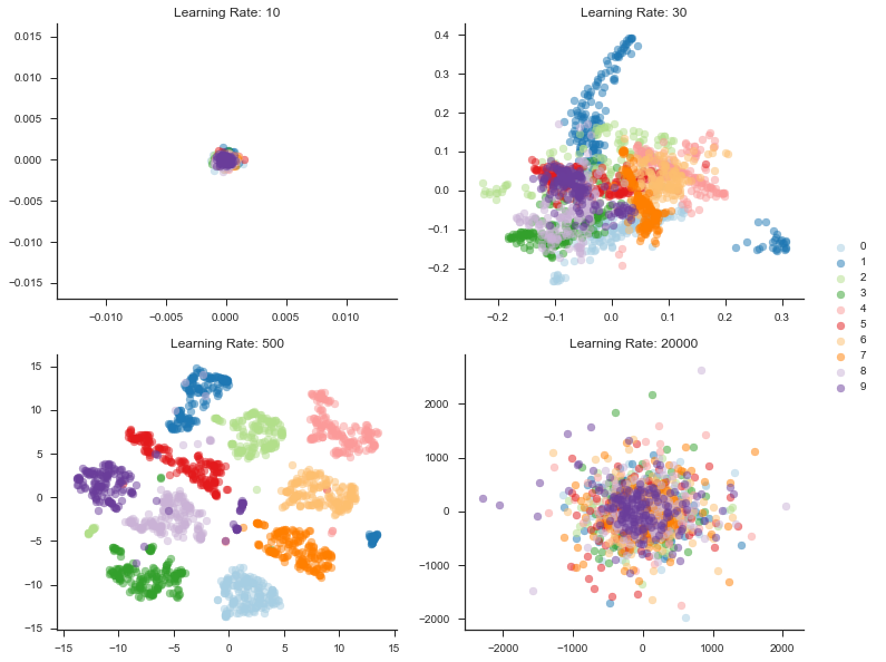
The learning rate for t-SNE is usually in the range [10.0, 1000.0]. If the learning rate is too high, the data may look like a ‘ball’ with any point approximately equidistant from its nearest neighbours. If the learning rate is too low, most points may look compressed in a dense cloud with few outliers. If the cost function gets stuck in a bad local minimum increasing the learning rate may help.

In these experiments, learning rate turned out to be a massively important hyperparameter as you can see below. Choosing a rate that is too low will fail to segment the space at all. Choosing one that is too large, will effectively scatter the points.

4. Iterations

n_iter : int, optional (default: 1000)

Maximum number of iterations for the optimization. Should be at least 250.

For this dataset, number of iterations really had no effect on the outcome. I even experimented with tuning down the learning rate, but that ended up just allowing the algorithm to hit a different steady state.

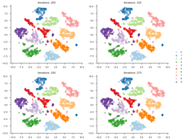
As you can see from the plot above, all plots are essentially the same. Interestingly, the error does decrease as we iterate. Just looking at the visualization, however, it is imperceivable. I experimented with large iterations–such as the default 1000 iterations–but the pattern does not change.

5. Random State

random_state : int, RandomState instance or None, optional (default: None)

If int, random_state is the seed used by the random number generator; If RandomState instance, random_state is the random number generator; If None, the random number generator is the RandomState instance used by np.random. Note that different initializations might result in different local minima of the cost function.

Random state is pretty straight forward. The algorithm just changes the initial projection. Interestingly, it always converges to roughly the same error.

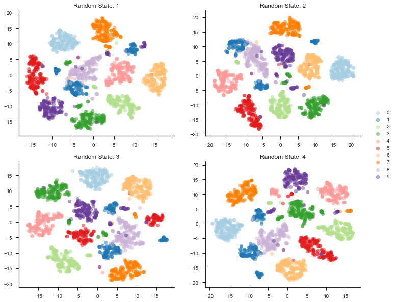
As we can see from the plot above, the random state greatly effects where each point will end up in the 2d space, but overall error and appearance remain pretty similar. One interesting thing is that nearby blobs are not guaranteed to be nearby in another random state. This is one of the tricky things about TSNE and make it difficult to interpret. For example, looking at random state 3 and random state 4, the red blobs are separated in random state 3, but form one large blob in random state 4.

6. Early Exaggeration

early_exaggeration : float, optional (default: 12.0)

Controls how tight natural clusters in the original space are in the embedded space and how much space will be between them. For larger values, the space between natural clusters will be larger in the embedded space. Again, the choice of this parameter is not very critical. If the cost function increases during initial optimization, the early exaggeration factor or the learning rate might be too high.

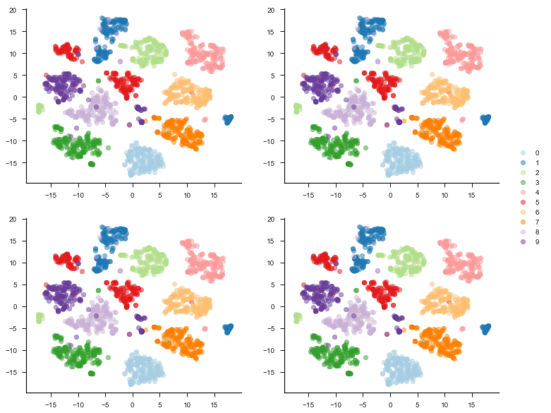
As we can see in the plot below, for this set of data, exaggeration has no effect on the final arrangement. The points ended up in about the same space with the exact same error.

Summary

Hopefully my experiments can be useful to your understanding of the TSNE algorithm. I find it extremely interesting and extremely useful.